
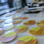


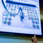


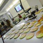


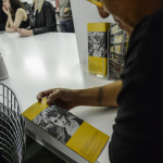


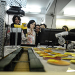
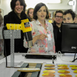

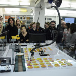

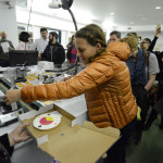


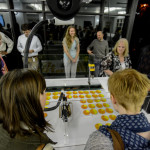
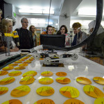
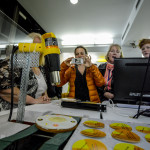
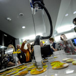
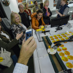


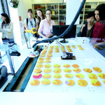
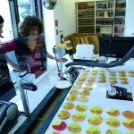
Pictures from the Feminist Data Collect-a-thon


Forward Kinematics, Inverse Kinematics, and the M100RAK Robot Arm
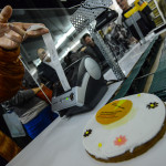
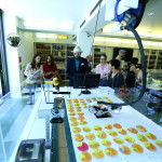
The video above shows the M100RAK drawing a rudimentary pie chart onto a pie with a “FoodWriter”, a marker containing food coloring. The pie chart depicts the gender ratio among Google’s staff (women: 30%, men 70%).
The food color marker does not draw well on chocolate, especially in hot weather. Tests with hard-drying royal icing and/or rice paper will follow.
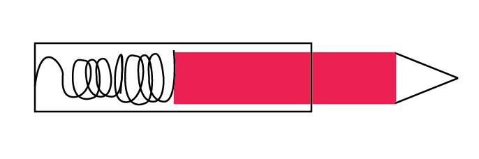
The marker is connected to aluminum piping with a spring. This means that it can draw on uneven surfaces.
The robot drawing itself is not yet optimal. If you compare it to the the perfectly round simulation below, you will see why.
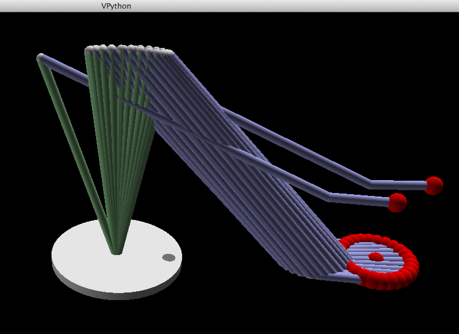
The simulation is made up of points that the robot connects. The two points that are floating above are not a mistake. They make sure that when the pen touches down, it touches down almost vertically. If these points were not there, the marker would leave a trail.
I don’t know yet why the robot draws more of a rectangle than a circle. It might be because the servos are slipping under the weight of the robot parts, or because I am falsely adapting the angles returned by the inverse kinematics function to the machine. The spacing between the gears is relatively wide, this might also negatively influence precision. In the meantime, here is an explanation of Inverse Kinematics and Forward Kinematics and how it relates to the code.
Kinematics & Forward Kinematics: The short explanation
Inverse Kinematics describes equations that produce angles to position a robotic arm on a specific xyz-coordinate. In other words: it is an algorithm (a function for example) that takes an xyz-coordinate as well as the length of the arm segments as parameters and returns the angles of the arm joints.
Forward Kinematics does the opposite. It takes angles and the length of the arm segments as inputs and then outputs an xyz-coordinate.
Inverse Kinematics and Forward Kinematics are used in robotics as well as in computer animation to animate objects in physical and in virtual spaces.
All the code in this project is in Python and requires the SciPy and vPython libraries for math and visualization respectively. It also requires the serial library for interfacing with the SC-32.
The Inverse Kinematics function in Python as well as a visualization function using vPython was written by Yaouen Fily specifically for this project.
Forward Kinematics
In order to get the arm to a certain point, we need an inverse kinematics function. However, to get there, it is easier to first derive the forward kinematics function. We will also need the forward kinematics function to draw the robot in 3D using vPython.
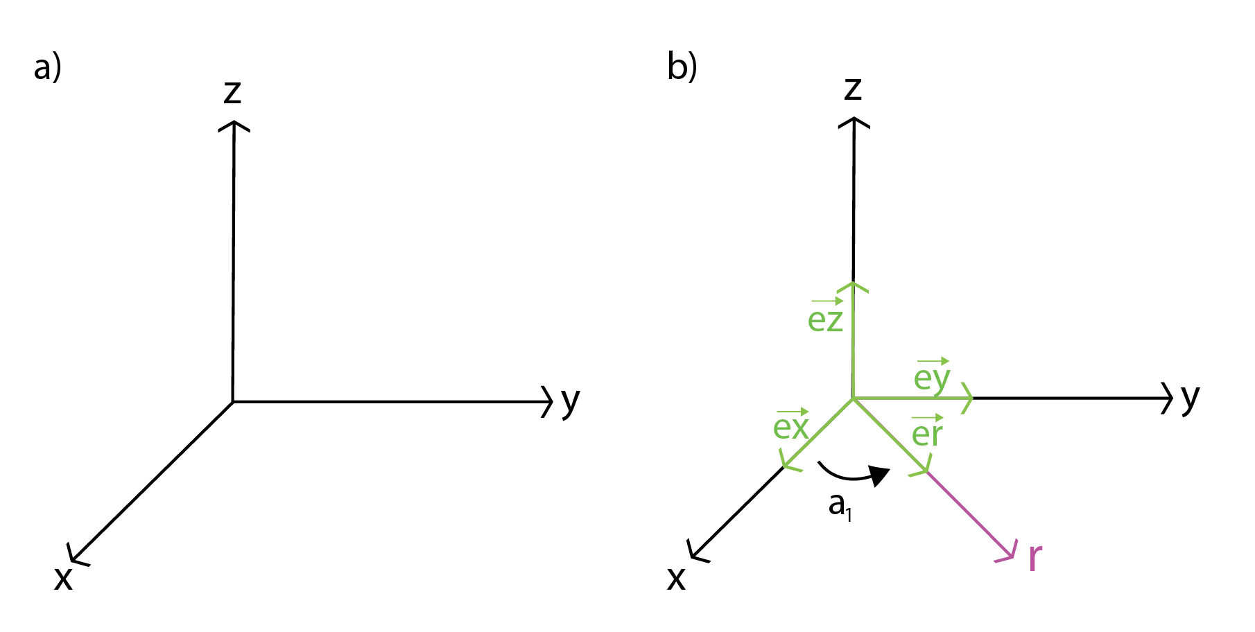
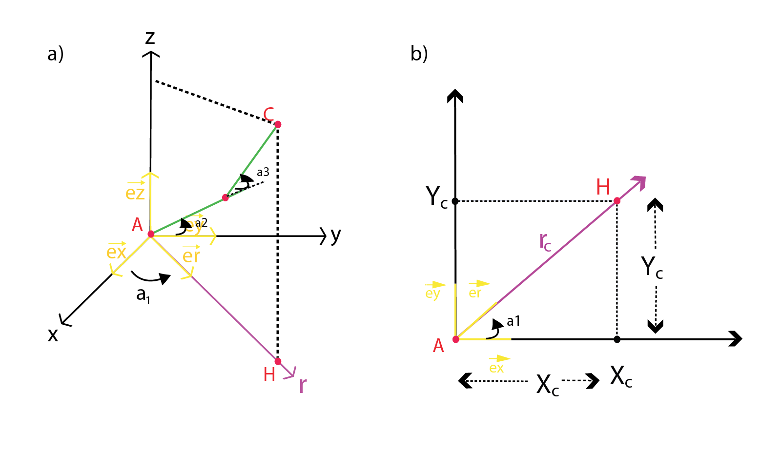
To get started, look at the image below. a) depicts a 3D space. b) depicts a 3D space with an additional direction r. The unit vectors on the xyz axes are  ,
,  ,
,  . Unit vectors are just vectors of length 1. Along r there is an additional unit vector
  with angle a1. Why is this vector important to our problem? Assuming that your targetThis could be the direction that the base of the robot arm rotates. This also makes things easier because now, we do not need the x and y axes anymore and can deal with this as a 2D trigonometry problem, not a 3D trigonometry problem in the following steps.
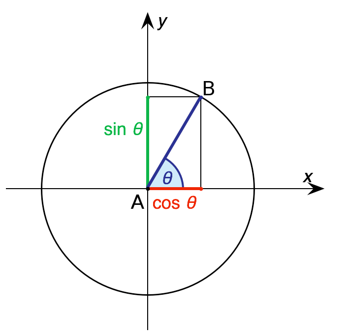
For the next step, look at the image below. It depicts a vector  of length 1 in a plane. makes an angle
  (theta) with the r axis. The r coordinate of the vector is
  , and its z coordinate is
  (see wikipedia for more detail). If the vector’s length is not 1, but some length AB, its r and z coordinates are
  and
and  instead.
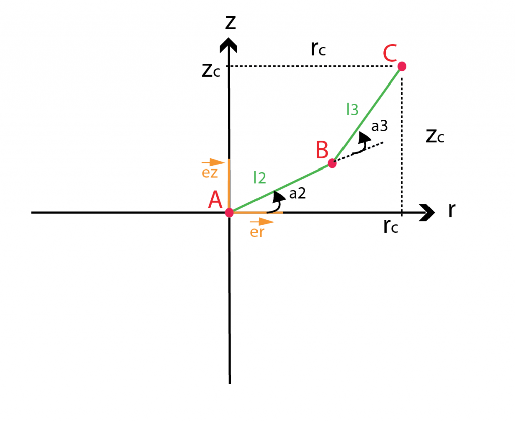
The next image (below) depicts our two axes, the z axis and the r axis as well as the unit vectors. It also depicts two new vectors  and
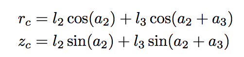
and  with length l2 and l3. These are the robot arm segments. A and B are the joints. C could be a joint as well if it had another segment attached (in the case of the M100RAK it does have an additional segment). Below are the forward kinematics equations. They give the coordinates of
  as functions of the arm lengths l2, l3 and joint angles a2 and a3.
The equation below describes the vector .
![\overrightarrow{AB} = l_2 \left[ \cos(a_2) \overrightarrow{e}_r + \sin(a_2) \overrightarrow{e}_z \right]](https://www.anninaruest.com/pie/wp-content/ql-cache/quicklatex.com-ad2b041570539317f290ec7938addfc8_l3.png "Rendered by QuickLaTeX.com")
The next equation describes the vector .
![\overrightarrow{BC} = l_3 \left[ \cos(a_2+a_3) \overrightarrow{e}_r + \sin(a_2+a_3) \overrightarrow{e}_z \right]](https://www.anninaruest.com/pie/wp-content/ql-cache/quicklatex.com-ba3e1da899329b9d4d4dd38e704fe16a_l3.png "Rendered by QuickLaTeX.com")
However what really interests us is the Vector since it tells us where the end of the arm will end up.
![\overrightarrow{AC} = \left[ l_2 \cos(a_2) + l_3 \cos(a_2+a_3) \right] \overrightarrow{e}_r + \left[ l_2 \sin(a_2) + l_3 \sin(a_2+a_3) \right] \overrightarrow{e}_z](https://www.anninaruest.com/pie/wp-content/ql-cache/quicklatex.com-c04dd9ee7069612fad793b95b7079a7b_l3.png "Rendered by QuickLaTeX.com")
If you are more of a coder than a mathematician, you can see this reflected in parts of the code. Specifically, in the function arms. The function takes angles a1, a2, a3 and a4 as well as the length of the arm segments as inputs and outputs a set of coordinates.
def arms(a1,a2,a3,a4,l2,l3,l4):
	er = cos(a1)*ex + sin(a1)*ey
	u2 = l2 * ( cos(a2)*er + sin(a2)*ez )
	u3 = l3 * ( cos(a2+a3)*er + sin(a2+a3)*ez )
	u4 = l4 * ( cos(a2+a3+a4)*er + sin(a2+a3+a4)*ez )
#	u4 = l4 * er
	return u2,u3,u4
You can also see it in the function draw_robot. In line 5, Yaouen calls invert, the inverse kinematics function to receive the angles of the arms. In line 6 he calls the arms function which does the forward kinematics. Both are necessary to draw the robot in 3D.
def draw_robot(x,y,z,l2,l3,l4):
	# first draw x,y,z axes
	p0 = 10*array([-1,-1,0])
	for e in ex,ey,ez:	vp.arrow(pos=p0,axis=5*e,shaftwidth=0.5,color=e)
	a1,a2,a3,a4 = invert(x,y,z,l2,l3,l4)                  # compute joint angles
	u2,u3,u4 = arms(a1,a2,a3,a4,l2,l3,l4)                    # compute arm vectors
	w = 0.2                                          # arm radius and base thickness
	u0 = w*ez
	v0 = cos(a1)*ex + sin(a1)*ey                     # "front" direction
	r = 3                                            # radius of the base
	vp.cylinder(pos=-u0,axis=2*u0,radius=r)         # draw base
	vp.cylinder(pos=-u0+0.8*r*v0,axis=2*u0,radius=0.1*r,color=(0.5,0.5,0.5)) # draw grey circle that indicates base direction
	vp.cylinder(pos=(0,0,0),axis=u2,radius=w,color=(0.7,1,0.7)) # draw arm 2
	vp.sphere(pos=u2,radius=w)                                  # draw joint 2
	vp.cylinder(pos=u2,axis=u3,radius=w,color=(0.7,0.7,1))      # draw arm 3
	vp.sphere(pos=u2+u3,radius=w)                               # draw joint 3
	vp.cylinder(pos=u2+u3,axis=u4,radius=w,color=(0.7,0.7,1))   # draw arm 4
	vp.sphere(pos=u2+u3+u4,radius=2*w,color=(0,1,0))            # draw end of arm 4
	vp.sphere(pos=(x,y,z),radius=2*w,color=(1,0,0))             # draw target point
	#the last two lines are doing the same but are there for debugging
Inverse Kinematics
Big picture: In order to get the end of the robot arm to point to an xyz-coordinate of our choice we need an inverse kinematics function. We also need the length of the arm segments. We can then give those two sets of parameters to the function and the function will calculate what angles we have to create between the arm segments (using motors). Below is an explanation of the math that Yaouen used to figure out how to to write the inverse kinematics function in Python. Its all trigonometry. However, this problem could also be solved using other mathematical methods.
Ok. Here we go: Below, you see the 3D space again. As previously said, we want to figure out angles as a function of arm lengths and an xyz coordinate. This coordinate is called C in the drawing below. To get started, we need to determine  ,
, , and
, and  . We can do this as a 2D problem as shown in b) by defining the point H which is a projection of C onto r.
This is the definition of 

This is the definition of 


Now that we have  and , the next step will be to determine AC and and
  .
.
The distance AC doesn’t depend on  , nor on
  , only on . Therefore computing AC will give us an equation that relates ,
  and
and  to
to  and
and  , that we can then solve for .
First we express AC in terms of the coordinates of C:


Then in terms of the arms lengths and joint angles, using the forward kinematics expressions from earlier:
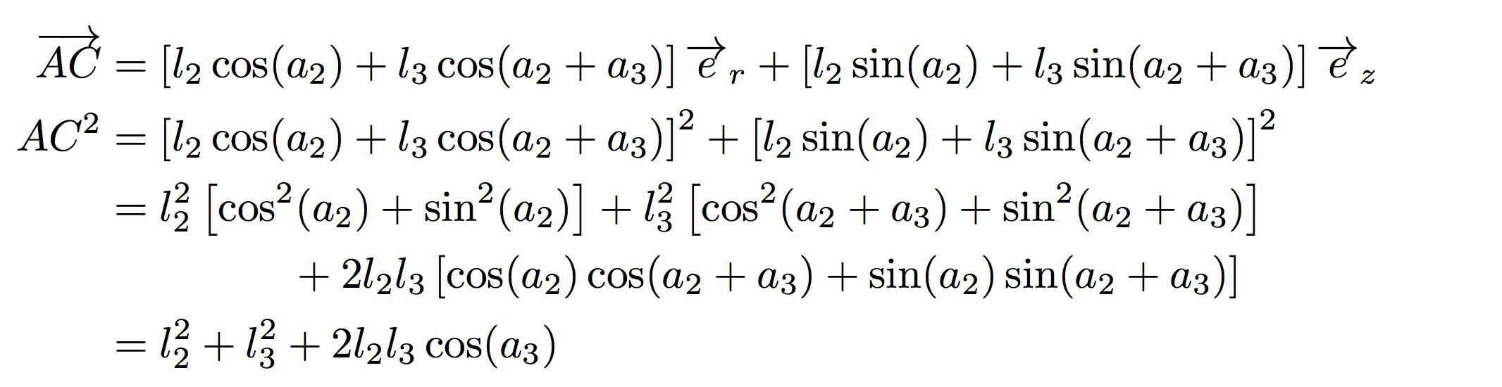
To get the last line we used the trigonometric relations (see wikipedia)

and

Comparing the two expressions of  , we get:
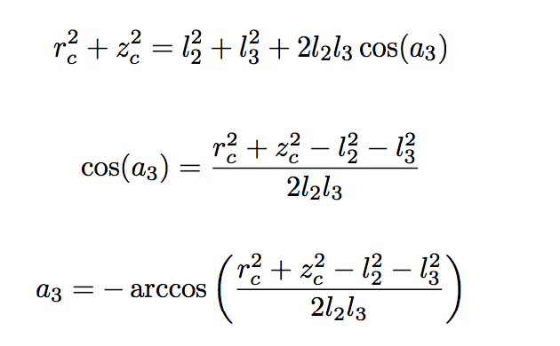
Look at the drawing below. It shows  , the “elbow” of the robot arm shown in green in a). In a) is negative. could in principle be positive or negative as shown in b). We chose the negative option because we do not want the arm to go below the base (the “shoulder” joint) and violently bang into the table as shown in c) (because the motors and everything else would suffer). Therefore we want B to be above C (B and C are shown in the previous images – not in the ones below).
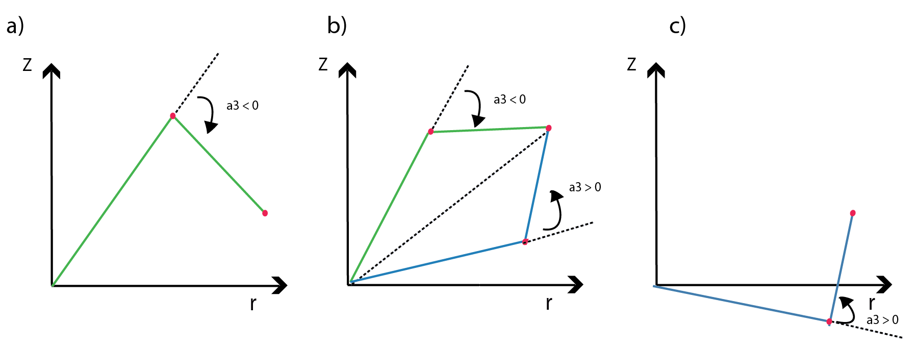
We want a3 to always be negative because else, the arm would be colliding with a surface below the table as shown in c).
Looking at the the two expressions of AC above, we can write
To disentangle  and , we now use the trigonometric formulae:
![]()
The result is:
![]()
If we now think cos( ) and sin( ) as two independent unknowns, this is a system of two linear equations, which can always be solved, using for example Cramer’s method (see wikipedia).
For the sake of notational brevity, we now introduce
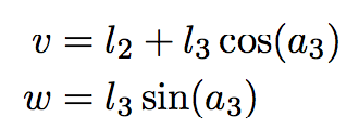
so that our equations can be shortened to:
![]()
On Wikipedia, the unknowns are x and y and the equations are:
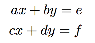
and the solution is:
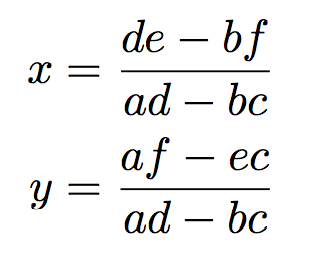
Using the following correspondence table:
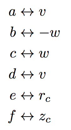
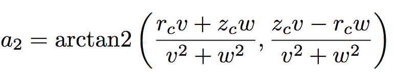
We obtain the solution to our equations:
Here is the function that does the inverse kinematics. You will see that it is similar to the math done in this section of the blog post:
# input: coordinates x,y,z of the target point, lengths b,c of the arms
# output: angles a1,a2,a3 of the joints, in degrees
def invert(x,y,z,l2,l3,l4):
s  = "(%g,%g,%g) is out of range." % tuple(around([x,y,z],2))
a1 = arctan2(y,x)
r  = hypot(x,y) - l4
u3 = ( r**2 + z**2 - l2**2 - l3**2 ) / ( 2*l2*l3 )
if abs(u3)>1:    raise Exception(s)
a3 = -arccos(u3)
v  = l2 + l3*u3
w  = -l3 * sqrt(1-u3**2)  # this is sin(a3), >0 assuming 0<a3<pi
a2 = arctan2(v*z-w*r,v*r+w*z)
#    # at this point a2<0 => take the other solution
#    a2 = 2*arctan2(z,r) - a2
#    a3 = -a3
if a2<0 or a2>pi:    raise Exception(s)
a4 = - a2 - a3
#    return r2d(a1,a2,a3)
return a1,a2,a3,a4
New Robot Arm
To make the next iteration of the project, I am currently working with the M100RAK V2 robot arm from Robotshop. The M100RAK is a step up from the OWI robotic arms that I used previously. It’s also roughly ten times more expensive if you also count the fact that the OWI arms require lots of modification to make them accurate enough.
The M100RAK (@$598) is intermediate-sized, this means that it has a reach of ~24inches at full extension. It has a similar reach to that of small industrial robotic arms. However, those are all more expensive (educational versions start at ~$3800) and (oftentimes) not as straightforward to operate.
The M100RAK V2 is shipped as a kit that needs to be assembled. Since the kit I received differs from the M100RAK V1, most of the parts are different and the kit did not yet seem ready to ship. The kit I received only included piping with 5/8″ diameter. I had to go to the hardware store to buy 1/2″ piping and cut it to size because certain fittings required the 1/2″ diameter. Some other stuff (such as the too-short shafts of the large gears) simply did not fit the designated components. However, this does not seem to affect the operation of the arm. I have no doubts that I assembled the robot arm correctly but was still left with lots of components that did not fit. This is obviously weird. I exchanged some messages with the Robotshop tech support. I did not implement the suggestions they made since they did not really make sense. In any case, I hope that they will improve the kit and the assembly instructions.
When the arm was assembled, I partially disassembled it and one by one connected three servos to the Lynxmotion SSC-32 servo controller and set them to position 1500 before re-assembling the arm. The SSC-32 can move up to 32 servos simultaneously (with appropriate power supply of course). And for somebody who’s been messing around with extremely low cost electronics before, the SSC-32 is a total luxury.
You can access SSC-32 via Python as follows:
import serial
ser = serial.Serial("/dev/tty.usbserial",115200)
ser.write("#0 P1500 #1 P1500 #2 P1490 T1000\r")
#0 is the first servo, #1 is the second servo, and #2 is the third servo. The positions where it is supposed to move are marked with a P. So in this example it is P1500, P1500, and P1490. T1000 means that it will complete the move in 1000 milliseconds (1 second). If you do not put this parameter, it will move at its fastest. This is relatively loud and abrupt. I prefer a more easy-going and quieter speed . The positions are more or less arbitrary (set by you), however, somewhere I read that P1500 is the middle. I found that 255-260 is about 90 degrees. So turning a a servo from the neutral position to about 90 degrees would require you to enter P1760.
The SSC-32 also has a command to tell you when it is busy and when it is not. This can be checked in a while loop in Python:
ser.write("#1 P1500 #2 P1500 T6000\r")
ser.write("Q\r")        #the command Q checks whether the machine is busy or not.
data = ser.read(1)      #this reads the first character of the serial response coming from SSC-32
while data == "+":      #if this character is a "+", the program will check again.
    ser.write("Q\r")    #are you done yet??
    data = ser.read(1)  #response
print "motion done!"    #if the motion is done, the response is "."
                        #and the program exits the while loop.
This is it for now. The next post will be about inverse kinematics using the M100RAK. It will be fun.